Natural Gradients in Practice

Download this notebook: natgrads.ipynb

This practical companion to Natural Gradients uses gpx.fit_natgrads and natural_gradient_step on two problems: Gaussian regression, where one step finds the variational optimum, and mini-batched Bernoulli classification, where we compare convergence and runtime with Adam. We finish by examining an unsafe step and the built-in backoff.

For the geometry and proofs, see the theory notebook. For an introduction to sparse variational GPs, start with stochastic sparse GPs. The dual sparse GP notebook applies the same ideas to site parameters.

# Enable Float64 for more stable matrix inversions.
import time

import equinox as eqx
import jax
from jax import config
import jax.numpy as jnp
import jax.random as jr
from jaxtyping import install_import_hook
import matplotlib as mpl
import matplotlib.pyplot as plt
import optax as ox
import paramax
from utils import clean_legend, use_mpl_style

config.update("jax_enable_x64", True)


with install_import_hook("gpjax", "beartype.beartype"):
    import gpjax as gpx
    import gpjax.kernels as jk
    from gpjax.natural_gradients import (
        expectation_from_moments,
        moments_from_expectation,
        natural_from_moments,
        natural_gradient_step,
        partition_variational,
    )
    from gpjax.parameters import LowerTriangular, Real, val

key = jr.key(123)

# set the default style for plotting
use_mpl_style()
cols = mpl.rcParams["axes.prop_cycle"].by_key()["color"]


def negative_elbo(model, data):
    """The loss every fit below minimises: GPJax optimisers descend, so negate."""
    return -gpx.objectives.elbo(model, data)

Gaussian regression: one step to the optimum

With a Gaussian likelihood, a natural-gradient step of size \(\gamma=1\) reaches the optimal \(q\) for fixed kernel and inducing inputs (Titsias [2009]). We check this against the closed-form solution, then compare with Adam from the same deliberately poor starting point.

num_data = 200
noise_stddev = 0.3

key, input_key, noise_key = jr.split(key, 3)
regression_inputs = jr.uniform(input_key, (num_data, 1), minval=-3.0, maxval=3.0)
regression_signal = jnp.sin(2.0 * regression_inputs)
regression_outputs = regression_signal + noise_stddev * jr.normal(
    noise_key, regression_signal.shape
)
regression_data = gpx.Dataset(X=regression_inputs, y=regression_outputs)

num_inducing = 20
regression_inducing = jnp.linspace(-3.0, 3.0, num_inducing).reshape(-1, 1)
test_inputs = jnp.linspace(-3.2, 3.2, 300).reshape(-1, 1)

# Keep the kernel fixed later so both optimisers solve the same variational
# problem.
regression_model = gpx.gps.Prior(
    mean_function=gpx.mean_functions.Constant(),
    kernel=jk.RBF(lengthscale=0.5),
    jitter=1e-8,
) * gpx.likelihoods.Gaussian(obs_stddev=noise_stddev)

key, bad_mean_key, bad_root_key = jr.split(key, 3)
bad_mean = jr.normal(bad_mean_key, (num_inducing, 1))
bad_factor = 0.3 * jr.normal(bad_root_key, (num_inducing, num_inducing))
bad_root = jnp.linalg.cholesky(bad_factor @ bad_factor.T + 0.5 * jnp.eye(num_inducing))

initial_family = gpx.variational_families.WhitenedVariationalGaussian(
    model=regression_model,
    inducing_inputs=regression_inducing,
    variational_mean=bad_mean,
    variational_root_covariance=bad_root,
)

The whitened family writes \(\mathbf{u}=\boldsymbol{\mu}_z+\mathbf{L}_z\mathbf{v}\) with a standard-normal prior on \(\mathbf{v}\). Its coordinate maps are the same as for an unwhitened Gaussian, but the variational parameters stay better scaled.

For \(\mathbf{A}_w=\mathbf{K}_{xz}\mathbf{L}_z^{-\top}\) and observation variance \(\sigma^2\), the reference optimum is

\[\boldsymbol{\Lambda}_w = \mathbf{I}_M + \sigma^{-2}\mathbf{A}_w^\top\mathbf{A}_w, \qquad \mathbf{b}_w = \sigma^{-2}\mathbf{A}_w^\top(\mathbf{y}-\boldsymbol{\mu}_x),\]

\[\mathbf{S}_w^\star = \boldsymbol{\Lambda}_w^{-1}, \qquad \mathbf{m}_w^\star = \boldsymbol{\Lambda}_w^{-1}\mathbf{b}_w .\]

kernel = initial_family.model.prior.kernel
mean_function = initial_family.model.prior.mean_function

Kzz = kernel.gram(regression_inducing).as_matrix()
Kzz = Kzz + initial_family.model.prior.jitter * jnp.eye(num_inducing)
Lz = jnp.linalg.cholesky(Kzz)
Kzx = kernel.cross_covariance(regression_inducing, regression_inputs)
whitened_design = jax.scipy.linalg.solve_triangular(Lz, Kzx, lower=True).T

observation_variance = noise_stddev**2
whitened_precision = (
    jnp.eye(num_inducing) + whitened_design.T @ whitened_design / observation_variance
)
whitened_shift = (
    whitened_design.T
    @ (regression_outputs - mean_function(regression_inputs))
    / observation_variance
)
optimal_covariance = jnp.linalg.inv(whitened_precision)
optimal_mean = jnp.linalg.solve(whitened_precision, whitened_shift)

# The ELBO at the closed-form optimum, used below as the reference for both
# methods.
optimal_family = eqx.tree_at(
    lambda family: (family.variational_mean, family.variational_root_covariance),
    initial_family,
    (Real(optimal_mean), LowerTriangular(jnp.linalg.cholesky(optimal_covariance))),
)
reference_elbo = float(gpx.objectives.elbo(optimal_family, regression_data))
print(f"ELBO at the closed-form optimum: {reference_elbo:.6f}")

ELBO at the closed-form optimum: -51.861140

# Split off the variational parameters; `natural_gradient_step` updates only
# that partition. `fit_natgrads` uses the same step internally.
variational_partition, hyper_partition = partition_variational(initial_family)
stepped_partition, loss_before = natural_gradient_step(
    variational_partition,
    hyper_partition,
    regression_data,
    negative_elbo,
    1.0,
    map_jitter=0.0,
)
stepped_family = eqx.combine(stepped_partition, hyper_partition)

stepped_mean = val(stepped_family.variational_mean)
stepped_root = val(stepped_family.variational_root_covariance)
stepped_covariance = stepped_root @ stepped_root.T

stepped_elbo = float(gpx.objectives.elbo(stepped_family, regression_data))

# A second step from the same place must be a fixed point.
twice_stepped_partition, _ = natural_gradient_step(
    stepped_partition,
    hyper_partition,
    regression_data,
    negative_elbo,
    1.0,
    map_jitter=0.0,
)
twice_stepped_mean = val(
    eqx.combine(twice_stepped_partition, hyper_partition).variational_mean
)

print(f"ELBO before the step           : {-loss_before:12.6f}")
print(f"ELBO after one gamma=1 step    : {stepped_elbo:12.6f}")
print(f"ELBO at the closed-form optimum: {reference_elbo:12.6f}")
print(
    "max |m_1 - m*|                 : "
    f"{jnp.max(jnp.abs(stepped_mean - optimal_mean)):.3e}"
)
print(
    "max |S_1 - S*|                 : "
    f"{jnp.max(jnp.abs(stepped_covariance - optimal_covariance)):.3e}"
)
print(
    "max |m_2 - m_1| (fixed point)  : "
    f"{jnp.max(jnp.abs(twice_stepped_mean - stepped_mean)):.3e}"
)

ELBO before the step           : -3084.291293
ELBO after one gamma=1 step    :   -51.861140
ELBO at the closed-form optimum:   -51.861140
max |m_1 - m*|                 : 9.479e-14
max |S_1 - S*|                 : 2.631e-14
max |m_2 - m_1| (fixed point)  : 9.136e-14

One step reaches the closed-form optimum; the second confirms it is a fixed point. map_jitter=0.0 avoids bias in the coordinate conversion. This is separate from Prior.jitter, which stabilises the inducing-point covariance.

How close is this sparse optimum to the full GP posterior?

exact_posterior = regression_model.condition(regression_data)
exact_predictive = exact_posterior(test_inputs)
exact_mean = exact_predictive.mean
exact_stddev = jnp.sqrt(exact_predictive.variance)

fig, axes = plt.subplots(ncols=2, figsize=(10, 3.0), sharey=True)
for ax, family, title in [
    (axes[0], initial_family, "Initialisation"),
    (axes[1], stepped_family, "After one $\\gamma=1$ natural-gradient step"),
]:
    predictive = family(test_inputs)
    predictive_mean = predictive.mean
    predictive_stddev = jnp.sqrt(predictive.variance)
    ax.scatter(
        regression_inputs,
        regression_outputs,
        alpha=0.2,
        s=8,
        color=cols[0],
        label="Observations",
    )
    ax.plot(
        test_inputs, exact_mean, color="black", linestyle="--", label="Exact posterior"
    )
    ax.fill_between(
        test_inputs.flatten(),
        exact_mean - 2 * exact_stddev,
        exact_mean + 2 * exact_stddev,
        alpha=0.15,
        color="black",
    )
    ax.plot(test_inputs, predictive_mean, color=cols[1], label="Variational $q$")
    ax.fill_between(
        test_inputs.flatten(),
        predictive_mean - 2 * predictive_stddev,
        predictive_mean + 2 * predictive_stddev,
        alpha=0.3,
        color=cols[1],
    )
    ax.set(xlabel=r"$x$", title=title, ylim=(-3.0, 3.0))
    clean_legend(ax)
axes[0].set_ylabel(r"$f(x)$")

Text(0, 0.5, '$f(x)$')

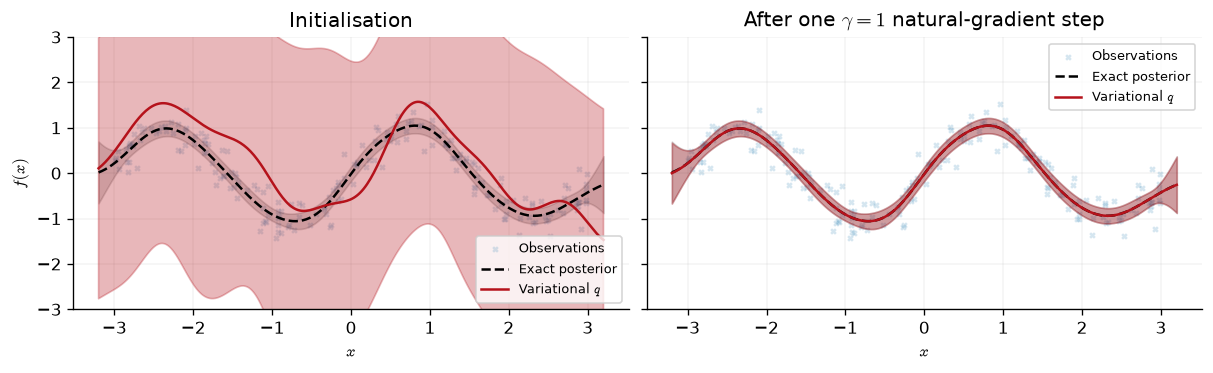
After one step, the sparse posterior is visually close to the exact GP. Any remaining gap comes from the inducing-point approximation, not from optimisation. To compare optimisers fairly, freeze the hyperparameters and run Adam on the same variational parameters from the same start.

frozen_family = eqx.combine(
    variational_partition, paramax.non_trainable(hyper_partition)
)

adam_iterations = 2000
_, adam_history = gpx.fit(
    model=frozen_family,
    objective=negative_elbo,
    train_data=regression_data,
    optim=ox.adam(1e-2),
    num_iters=adam_iterations,
    key=jr.key(0),
    verbose=False,
)

adam_gap = jnp.asarray(adam_history) + reference_elbo
natgrad_gap = reference_elbo - stepped_elbo
iteration_index = jnp.arange(adam_gap.size)
print(f"Adam's final ELBO gap after {adam_iterations} steps: {float(adam_gap[-1]):.3e}")
print(f"Natural-gradient gap after one step: {natgrad_gap:.3e}")

fig, ax = plt.subplots(figsize=(6, 3))
ax.plot(
    iteration_index + 1, jnp.maximum(adam_gap, 1e-16), color=cols[0], label="Adam"
)
ax.scatter(
    [1], [max(natgrad_gap, 1e-16)], color=cols[1], label="Natural gradient"
)
ax.set(xscale="log", yscale="log", xlabel="Iteration", ylabel="ELBO gap (nats)")
clean_legend(ax)

Adam's final ELBO gap after 2000 steps: 6.001e-01
Natural-gradient gap after one step: -7.105e-15

<Axes: xlabel='Iteration', ylabel='ELBO gap (nats)'>

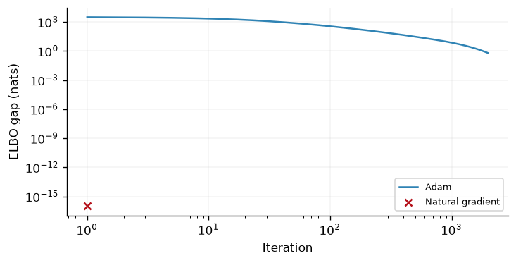
The natural gradient closes the ELBO gap in one step. Adam continues to improve after 2,000 steps but has not reached that optimum. This is a particularly favourable comparison for natural gradients: the kernel is frozen and the likelihood is conjugate. Neither condition holds next.

Banana classification: iterations and time

Outside conjugacy, \(\gamma=1\) is a local step, not an exact solve. Mini-batches also make its target noisy. We ramp \(\gamma\) from \(10^{-4}\) to \(10^{-1}\) over 100 iterations with an Optax schedule passed as natgrad_lr, while Adam updates the kernel and inducing inputs. A smaller step averages successive mini-batch targets rather than jumping directly to each one. The theory notebook explains the update.

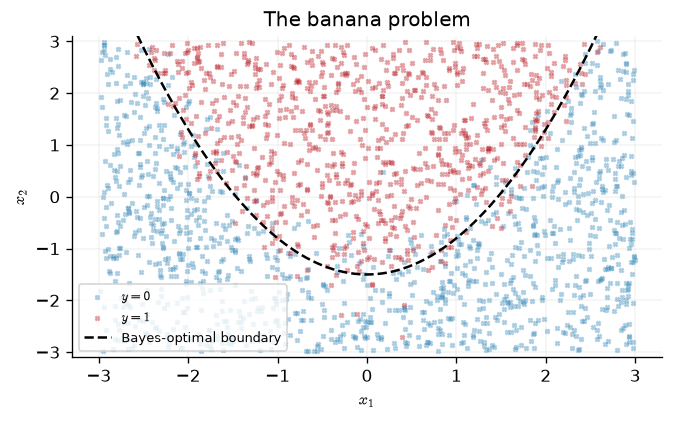
def make_banana(key, num_points):
    """Two-class banana problem with a curved Bayes-optimal boundary."""
    key_latent, key_label = jr.split(key)
    latent = jr.uniform(key_latent, (num_points, 2), minval=-3.0, maxval=3.0)
    decision = latent[:, 1] - (0.7 * latent[:, 0] ** 2 - 1.5)
    probability = jax.nn.sigmoid(3.0 * decision)
    labels = (jr.uniform(key_label, (num_points,)) < probability).astype(jnp.float64)
    return latent, labels[:, None]


banana_key = jr.key(42)
banana_inputs, banana_labels = make_banana(banana_key, 2000)
banana_data = gpx.Dataset(X=banana_inputs, y=banana_labels)

num_train = 1600
train_inputs, test_inputs_2d = banana_inputs[:num_train], banana_inputs[num_train:]
train_labels, test_labels = banana_labels[:num_train], banana_labels[num_train:]
banana_train = gpx.Dataset(X=train_inputs, y=train_labels)

print(f"train / test  : {banana_train.n} / {banana_data.n - banana_train.n}")
print(f"class balance : {float(banana_data.y.mean()):.3f}")

train / test  : 1600 / 400
class balance : 0.420

boundary_inputs = jnp.linspace(-3.0, 3.0, 200)
boundary_outputs = 0.7 * boundary_inputs**2 - 1.5

fig, ax = plt.subplots(figsize=(5.5, 3.4))
for label, colour, name in [(0.0, cols[0], "$y = 0$"), (1.0, cols[1], "$y = 1$")]:
    mask = banana_labels.ravel() == label
    ax.scatter(
        banana_inputs[mask, 0],
        banana_inputs[mask, 1],
        s=6,
        alpha=0.4,
        color=colour,
        label=name,
    )
ax.plot(
    boundary_inputs,
    boundary_outputs,
    color="black",
    linestyle="--",
    label="Bayes-optimal boundary",
)
ax.set(xlabel=r"$x_1$", ylabel=r"$x_2$", ylim=(-3.1, 3.1), title="The banana problem")
clean_legend(ax)

# Both runs use the same inducing grid and starting distribution.
num_banana_inducing = 50
inducing_grid = jnp.meshgrid(jnp.linspace(-2.8, 2.8, 10), jnp.linspace(-2.8, 2.8, 5))
banana_inducing = jnp.stack([axis.ravel() for axis in inducing_grid], axis=1)

banana_model = (
    gpx.gps.Prior(
        mean_function=gpx.mean_functions.Zero(), kernel=jk.RBF(active_dims=[0, 1])
    )
    * gpx.likelihoods.Bernoulli()
)


def make_banana_family():
    """A fresh SVGP over the banana data, at the default m = 0, S = I."""
    return gpx.variational_families.VariationalGaussian(
        model=banana_model, inducing_inputs=banana_inducing
    )


natgrad_family = make_banana_family()
adam_family = make_banana_family()

print(f"inducing inputs: {banana_inducing.shape}")

inducing inputs: (50, 2)

# The log-linear ramp, 1e-4 -> 1e-1 over K = 100 iterations, as an Optax
# schedule handed straight to `natgrad_lr`.
num_iterations = 1000
batch_size = 256
natgrad_schedule = ox.exponential_decay(
    init_value=1e-4, transition_steps=100, decay_rate=1000.0, end_value=1e-1
)


def timed_fit(run):
    """Run twice: the first call pays JIT compilation, the second is steady state."""
    model, history = run()
    history.block_until_ready()
    start = time.perf_counter()
    model, history = run()
    history.block_until_ready()
    return model, history, time.perf_counter() - start

natgrad_model, natgrad_history, natgrad_seconds = timed_fit(
    lambda: gpx.fit_natgrads(
        model=natgrad_family,
        objective=negative_elbo,
        train_data=banana_train,
        optim=ox.adam(1e-2),
        natgrad_lr=natgrad_schedule,
        batch_size=batch_size,
        num_iters=num_iterations,
        key=jr.key(1),
        verbose=False,
    )
)
print(
    f"natural gradients + Adam : {natgrad_seconds:.2f} s "
    f"({1e3 * natgrad_seconds / num_iterations:.2f} ms / iteration)"
)

natural gradients + Adam : 7.55 s (7.55 ms / iteration)

adam_model, adam_banana_history, adam_seconds = timed_fit(
    lambda: gpx.fit(
        model=adam_family,
        objective=negative_elbo,
        train_data=banana_train,
        optim=ox.adam(1e-2),
        batch_size=batch_size,
        num_iters=num_iterations,
        key=jr.key(1),
        verbose=False,
    )
)
print(
    f"Adam only                : {adam_seconds:.2f} s "
    f"({1e3 * adam_seconds / num_iterations:.2f} ms / iteration)"
)

Adam only                : 4.68 s (4.68 ms / iteration)

Both runs use Adam on the kernel and inducing inputs; only the variational update differs. Timings exclude compilation (the second of two identical runs is timed) and depend on the machine.

smoothing_window = 25


def smooth(history):
    """Trailing mean over `smoothing_window` iterations."""
    return jnp.convolve(
        history, jnp.ones(smoothing_window) / smoothing_window, mode="valid"
    )


smoothed_iterations = jnp.arange(smoothing_window - 1, num_iterations)
smoothed_natgrad = smooth(natgrad_history)
smoothed_adam = smooth(adam_banana_history)

# Derive the axis limits from the curves, so nothing is silently clipped on a
# machine whose run lands somewhere else.
elbo_floor = 0.95 * float(jnp.minimum(smoothed_natgrad.min(), smoothed_adam.min()))
elbo_ceiling = 1.10 * float(jnp.maximum(smoothed_natgrad.max(), smoothed_adam.max()))

fig, axes = plt.subplots(ncols=2, figsize=(10, 3.0), sharey=True)
for ax, horizontal, xlabel in [
    (axes[0], smoothed_iterations, "Iteration"),
    (
        axes[1],
        jnp.linspace(0.0, natgrad_seconds, num_iterations)[smoothing_window - 1 :],
        "Wall-clock seconds",
    ),
]:
    ax.plot(
        horizontal, smoothed_natgrad, color=cols[1], label="Natural gradients + Adam"
    )
    ax.set(xlabel=xlabel, yscale="log", ylim=(elbo_floor, elbo_ceiling))
axes[0].plot(smoothed_iterations, smoothed_adam, color=cols[0], label="Adam only")
axes[1].plot(
    jnp.linspace(0.0, adam_seconds, num_iterations)[smoothing_window - 1 :],
    smoothed_adam,
    color=cols[0],
    label="Adam only",
)
axes[0].set_ylabel("Negative ELBO (mini-batch)")
clean_legend(axes[0])
clean_legend(axes[1])

# Compare when natural gradients first beat Adam's final smoothed loss.
target_value = float(smoothed_adam[-1])
never = num_iterations + 1
crossing = int(
    jnp.min(jnp.where(smoothed_natgrad < target_value, smoothed_iterations, never))
)
print(f"Adam final negative ELBO: {target_value:.2f}")
print(f"Natural-gradient final negative ELBO: {float(smoothed_natgrad[-1]):.2f}")
if crossing != never:
    print(
        f"Natural gradients reach Adam's final value at step {crossing} "
        f"({crossing * natgrad_seconds / num_iterations:.2f} s vs "
        f"{adam_seconds:.2f} s for Adam)"
    )
else:
    print("Natural gradients do not reach Adam's final value")

Adam final negative ELBO: 335.31
Natural-gradient final negative ELBO: 323.98
Natural gradients reach Adam's final value at step 117 (0.88 s vs 4.68 s for Adam)

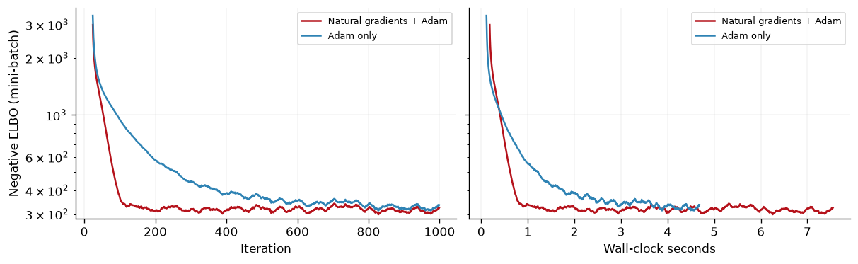
The curves show a 25-step trailing mean of noisy mini-batch losses. Compare both iteration count and elapsed time: a natural-gradient step costs more than an Adam step, so these rankings need not agree.

for name, model in [
    ("Natural gradients + Adam", natgrad_model),
    ("Adam only", adam_model),
]:
    probability = model.model.likelihood(model(test_inputs_2d)).mean
    labels = test_labels.ravel()
    accuracy = jnp.mean((probability > 0.5) == (labels > 0.5))
    nlpd = -jnp.mean(
        labels * jnp.log(probability) + (1 - labels) * jnp.log1p(-probability)
    )
    print(f"{name}: test accuracy {accuracy:.3f}, NLPD {nlpd:.3f}")

Natural gradients + Adam: test accuracy 0.935, NLPD 0.166
Adam only: test accuracy 0.933, NLPD 0.169

The held-out metrics are similar: faster optimisation here does not yield a clear predictive-quality gain. Both methods also update the kernel and inducing inputs, so the final models differ in more than their variational parameters.

Step sizes and backoff

The covariance requires \(\boldsymbol{\Theta}_2=-\tfrac12\mathbf{S}^{-1}\) to remain negative definite. For a log-concave likelihood, the cone-safety result guarantees this when \(0\le\gamma\le1\), even with mini-batches. Larger steps can overshoot. GPJax’s clipped Bernoulli link is not log-concave in its far tails, so it falls outside that guarantee there. We start from an overconfident covariance \(\mathbf{S}_0=10^{-2}\mathbf{I}\) to show an overshoot.

overconfident_family = gpx.variational_families.VariationalGaussian(
    model=banana_model,
    inducing_inputs=banana_inducing,
    variational_mean=jnp.zeros((num_banana_inducing, 1)),
    variational_root_covariance=0.1 * jnp.eye(num_banana_inducing),
)
overconfident_mean = val(overconfident_family.variational_mean)
overconfident_root = val(overconfident_family.variational_root_covariance)


def banana_loss_of_expectation(expectation):
    variational_mean, variational_root = moments_from_expectation(*expectation)
    trial = eqx.tree_at(
        lambda family: (family.variational_mean, family.variational_root_covariance),
        overconfident_family,
        (Real(variational_mean), LowerTriangular(variational_root)),
    )
    return negative_elbo(trial, banana_train)


cone_gradient = jax.grad(banana_loss_of_expectation)(
    expectation_from_moments(overconfident_mean, overconfident_root)
)
# The matrix statistic is symmetric, so symmetrise the entrywise autodiff
# gradient.
matrix_gradient = 0.5 * (cone_gradient[1] + cone_gradient[1].T)
_, natural_matrix = natural_from_moments(overconfident_mean, overconfident_root)

print("gamma      max eig(Theta2_new)   status")
for gamma in [0.1, 0.5, 1.0, 2.0, 5.0, 10.0]:
    largest = jnp.max(jnp.linalg.eigvalsh(natural_matrix - gamma * matrix_gradient))
    status = "negative definite" if largest < 0 else "*** LEFT THE CONE ***"
    print(f"{gamma:6.2f}   {largest:+18.5f}   {status}")

gamma      max eig(Theta2_new)   status
  0.10            -45.46684   negative definite
  0.50            -27.33418   negative definite
  1.00             -4.66836   negative definite
  2.00            +40.66328   *** LEFT THE CONE ***
  5.00           +176.65821   *** LEFT THE CONE ***
 10.00           +403.31642   *** LEFT THE CONE ***

For this start, \(\gamma=1\) remains inside the cone but \(\gamma=2\) does not. The crossing point is specific to this start, not a universal threshold. natural_gradient_step tries smaller rates when Cholesky fails: backoff defaults to \(0.5\) and max_backoff to five reductions.

print("gamma = 100 from the over-confident initialisation")
overconfident_variational, overconfident_hyper = partition_variational(
    overconfident_family
)
for max_backoff in [0, 3, 5, 7, 10]:
    stepped, _ = natural_gradient_step(
        overconfident_variational,
        overconfident_hyper,
        banana_train,
        negative_elbo,
        100.0,
        max_backoff=max_backoff,
    )
    smallest_trial = 100.0 * 0.5**max_backoff
    root = val(
        eqx.combine(stepped, overconfident_hyper).variational_root_covariance
    )
    outcome = "finite" if bool(jnp.all(jnp.isfinite(root))) else "NaN"
    print(
        f"  max_backoff = {max_backoff:2d}  smallest trial gamma = "
        f"{smallest_trial:7.3f}   result: {outcome}"
    )

gamma = 100 from the over-confident initialisation
  max_backoff =  0  smallest trial gamma = 100.000   result: NaN
  max_backoff =  3  smallest trial gamma =  12.500   result: NaN
  max_backoff =  5  smallest trial gamma =   3.125   result: NaN
  max_backoff =  7  smallest trial gamma =   0.781   result: finite
  max_backoff = 10  smallest trial gamma =   0.098   result: finite

Backoff has a finite budget. Here \(\gamma=100\) needs seven halvings; the default five still return NaN. Choose a sensible rate rather than relying on backoff to repair an overshoot.

Practical guidance

• Conjugate, full batch: \(\gamma=1\) reaches the variational optimum for fixed hyperparameters.

• Non-conjugate or mini-batched: start small and ramp natgrad_lr with an Optax schedule. A larger batch can reduce stochastic noise.

• Stay at or below \(\gamma=1\): outside that range there is no general cone-safety guarantee; backoff is a fallback, not a learning-rate policy.

• Whiten when conditioning is poor: the distributional update is unchanged in exact arithmetic, but coordinate maps are better scaled. Leave map_jitter at zero unless those maps need stabilising.

• Check likelihood curvature: non-log-concave likelihoods (including GPJax’s clipped Bernoulli in its tails) lack the general safety guarantee even below \(\gamma=1\).

System configuration

%reload_ext watermark
%watermark -n -u -v -iv -w -a 'Thomas Pinder'

Author: Thomas Pinder

Last updated: Mon, 28 Sep 2026

Python implementation: CPython
Python version       : 3.11.16
IPython version      : 9.17.1

equinox   : 0.13.8
gpjax     : 1.0.0
jax       : 0.10.2
jaxtyping : 0.3.11
matplotlib: 3.11.2
optax     : 0.2.8
paramax   : 0.0.5

Watermark: 2.6.0