Backend Module Design#
Download this notebook: backend.ipynb
GPJax is built upon Equinox and Paramax. Equinox provides a lightweight module system for JAX, whilst Paramax adds support for constrained parameters via unwrappable types. This notebook provides a high-level overview of the backend module design in GPJax. For an introduction to Equinox, please refer to the official documentation.
import typing as tp

import equinox as eqx
from utils import use_mpl_style
from gpjax.mean_functions import (
    AbstractMeanFunction,
    Constant,
)
from gpjax.parameters import (
    PositiveReal,
    Real,
    val,
)
from gpjax.typing import (
    Array,
    ScalarFloat,
)

# Enable Float64 for more stable matrix inversions.
from jax import config
import jax.numpy as jnp
import jax.tree_util as jtu
from jaxtyping import (
    Float,
    Num,
    install_import_hook,
)
import matplotlib as mpl
import matplotlib.pyplot as plt
try:
    from myst_nb import glue
except ImportError:  # notebook downloaded and run outside the docs build
    def glue(*args, **kwargs):
        """No-op stand-in: gluing only matters when Sphinx renders this page."""
from paramax import AbstractUnwrappable

config.update("jax_enable_x64", True)


with install_import_hook("gpjax", "beartype.beartype"):
    import gpjax as gpx


# set the default style for plotting
use_mpl_style()

cols = mpl.rcParams["axes.prop_cycle"].by_key()["color"]
Parameters#
GPJax uses Paramax to handle constrained
parameters. As discussed in our Sharp Bits -
Bijectors Doc, GPJax
uses bijectors to transform constrained parameters to unconstrained parameters during
optimisation. You may register the support of a parameter using our parameter types.
To see this, consider the Constant mean function which
contains a single constant
parameter whose value ordinarily exists on the real line. We can register this
parameter as follows:
constant_param = Real(1.0)
meanf = Constant(constant_param)
print(meanf)
Constant(constant=Real(value=weak_f64[]))
However, suppose you wish your mean function’s constant parameter to be strictly
positive. This is easy to achieve by using the correct parameter type which, in this
case, will be the PositiveReal. All parameter types are
subclasses of Paramax’s
AbstractUnwrappable, which means they
will be automatically transformed by GPJax
during optimisation.
isinstance(PositiveReal(1.0), AbstractUnwrappable)
True
Injecting this newly constrained parameter into our mean function is then identical to before.
constant_param = PositiveReal(value=1.0)
meanf = Constant(constant_param)
print(meanf)
Constant(constant=PositiveReal(_unconstrained=weak_f64[]))
Parameter Transforms#
With a parameter instantiated, you likely wish to transform the parameter’s value from
its constrained support onto the entire real line. In GPJax, parameters store their
values internally in unconstrained space. When you need the constrained value, call
val on the parameter.
Constrained value: 1.0
Unconstrained (internal) value: 0.5413248546129181
We see here that the Softplus bijector is applied by the PositiveReal parameter type.
Internally, the value 1.0 is stored as its inverse-softplus
(~0.54), and calling
val applies softplus to recover the original constrained value.
val is the single rule you need to remember: models are always held in their
wrapped form — the model you build, and the model fit hands back — and val is
what you call at the point where a parameter meets arithmetic. It is safe to apply to
anything, returning plain arrays and floats untouched, so there is never a need to
check whether a value is wrapped first.
For a value closer to 0, the transformation is more pronounced.
Transforming Multiple Parameters#
In the above, we transformed a single parameter. However, in practice your parameters may be nested within several functions e.g., a kernel function within a GP model. Fortunately, transforming several parameters is a simple operation that we here demonstrate for a conjugate GP posterior (see our Regression Notebook for detailed explanation of this model.).
kernel = gpx.kernels.Matern32()
meanf = gpx.mean_functions.Constant()

prior = gpx.gps.Prior(mean_function=meanf, kernel=kernel)

likelihood = gpx.likelihoods.Gaussian()
posterior = likelihood * prior
print(posterior)
ConjugateModel(
  prior=Prior(
    kernel=Matern32(
      active_dims=slice(None, None, None),
      compute_engine=<gpjax.kernels.computations.dense.DenseKernelComputation object at 0x7febe81a5ed0>,
      lengthscale=PositiveReal(_unconstrained=weak_f64[]),
      variance=NonNegativeReal(_unconstrained=weak_f64[])
    ),
    mean_function=Constant(constant=weak_f64[])
  ),
  likelihood=Gaussian(
    integrator=<gpjax.integrators.AnalyticalGaussianIntegrator object at 0x7febe0342cd0>,
    obs_stddev=NonNegativeReal(_unconstrained=weak_f64[])
  )
)
Summarising a model#
The print(posterior) output above is Equinox’s representation: it exposes each
parameter’s unconstrained internal storage and conveys nothing about bijectors or
trainability. For a human-readable overview, use
gpx.summarise, which renders a flat
table — one row per parameter — showing the constrained value, the bijector, whether
the parameter is trainable, and its shape and dtype. It works on any GPJax model: a
kernel, prior, posterior, likelihood, or variational family.
gpx.summarise(posterior)
ConjugateModel
╭──────────────────────────────┬─────────────────┬───────┬──────────┬───────┬───────────┬───────┬───────╮
│ Parameter                    │ Class           │ Value │ Bijector │ Prior │ Trainable │ Shape │ Dtype │
├──────────────────────────────┼─────────────────┼───────┼──────────┼───────┼───────────┼───────┼───────┤
│ prior.kernel.lengthscale     │ PositiveReal    │ 1     │ Softplus │ -     │ yes       │ ()    │ f64   │
│ prior.kernel.variance        │ NonNegativeReal │ 1     │ Softplus │ -     │ yes       │ ()    │ f64   │
│ prior.mean_function.constant │ Array           │ 0     │ Identity │ -     │ yes       │ ()    │ f64   │
│ likelihood.obs_stddev        │ NonNegativeReal │ 1     │ Softplus │ -     │ yes       │ ()    │ f64   │
╰──────────────────────────────┴─────────────────┴───────┴──────────┴───────┴───────────┴───────┴───────╯
4 parameters, 4 trainable
summarise traverses the model as a PyTree, so composite objects (e.g. sum kernels)
and frozen parameters are handled automatically — frozen rows are dimmed and reported
as non-trainable. The same table backs rich.print(posterior) and Jupyter’s automatic
display, whilst repr(posterior) is left untouched.
Now contained within the posterior there are four parameters: the kernel’s lengthscale
and variance, the noise variance of the likelihood, and the constant of the mean
function. With Equinox, we can partition the model into its array leaves and static
structure using eqx.partition. This gives us direct access to the parameters as a
PyTree.
params, static = eqx.partition(posterior, eqx.is_array)
print(params)
ConjugateModel(
  prior=Prior(
    kernel=Matern32(
      active_dims=slice(None, None, None),
      compute_engine=<gpjax.kernels.computations.dense.DenseKernelComputation object at 0x7febe81a5ed0>,
      lengthscale=PositiveReal(_unconstrained=weak_f64[]),
      variance=NonNegativeReal(_unconstrained=weak_f64[])
    ),
    mean_function=Constant(constant=weak_f64[])
  ),
  likelihood=Gaussian(
    integrator=<gpjax.integrators.AnalyticalGaussianIntegrator object at 0x7febe0342cd0>,
    obs_stddev=NonNegativeReal(_unconstrained=weak_f64[])
  )
)
The params object behaves just like a PyTree and, consequently, we may use JAX’s
tree_map function to alter the values. The updated params can then be recombined
with the static structure using eqx.combine. In the below, we increment each leaf
by 1.
updated_params = jtu.tree_map(lambda x: x + 1, params)
print(updated_params)
ConjugateModel(
  prior=Prior(
    kernel=Matern32(
      active_dims=slice(None, None, None),
      compute_engine=<gpjax.kernels.computations.dense.DenseKernelComputation object at 0x7febe81a5ed0>,
      lengthscale=PositiveReal(_unconstrained=weak_f64[]),
      variance=NonNegativeReal(_unconstrained=weak_f64[])
    ),
    mean_function=Constant(constant=weak_f64[])
  ),
  likelihood=Gaussian(
    integrator=<gpjax.integrators.AnalyticalGaussianIntegrator object at 0x7febe0342cd0>,
    obs_stddev=NonNegativeReal(_unconstrained=weak_f64[])
  )
)
Note what eqx.partition handed us: the array leaves are the parameters’
unconstrained internals (lengthscale._unconstrained rather than lengthscale),
so tree_map operates in unconstrained space. Adding 1 to the leaf of a
unit lengthscale gives a constrained value of ~1.74, not 2.0, because the increment
lands before the softplus. This is exactly the behaviour optimisation depends on —
gradient steps are taken in the unconstrained space — but it does mean tree-mapping
arithmetic over a model is not a way to set parameter values. To do that, construct
a new parameter and swap it in with
eqx.tree_at.
Let us now use Equinox’s combine function to reconstruct the posterior distribution
using the updated parameters.
updated_posterior = eqx.combine(updated_params, static)
print(updated_posterior)
ConjugateModel(
  prior=Prior(
    kernel=Matern32(
      active_dims=slice(None, None, None),
      compute_engine=<gpjax.kernels.computations.dense.DenseKernelComputation object at 0x7febe81a5ed0>,
      lengthscale=PositiveReal(_unconstrained=weak_f64[]),
      variance=NonNegativeReal(_unconstrained=weak_f64[])
    ),
    mean_function=Constant(constant=weak_f64[])
  ),
  likelihood=Gaussian(
    integrator=<gpjax.integrators.AnalyticalGaussianIntegrator object at 0x7febe0342cd0>,
    obs_stddev=NonNegativeReal(_unconstrained=weak_f64[])
  )
)
To read a constrained parameter value out of the model, reach for val at the point
of use. Note that there is no separate step converting the model into some other
form: posterior is the same wrapped object throughout, whether you are inspecting
it, evaluating an objective on it, or passing it to fit. For a view of every
parameter at once, use gpx.summarise as above.
Fine-Scale Control#
One of the advantages of Equinox’s partition mechanism is that we can gain fine-scale
control over which parameters we extract. For example, suppose we only wish to extract
those parameters whose support is the positive real line. This is easily achieved by
providing a custom filter function to eqx.partition.
positive_reals, other_params = eqx.partition(
    posterior, lambda leaf: isinstance(leaf, PositiveReal)
)
print(positive_reals)
ConjugateModel(
  prior=Prior(
    kernel=Matern32(
      active_dims=slice(None, None, None),
      compute_engine=<gpjax.kernels.computations.dense.DenseKernelComputation object at 0x7febe81a5ed0>,
      lengthscale=PositiveReal(_unconstrained=None),
      variance=NonNegativeReal(_unconstrained=None)
    ),
    mean_function=Constant(constant=None)
  ),
  likelihood=Gaussian(
    integrator=<gpjax.integrators.AnalyticalGaussianIntegrator object at 0x7febe0342cd0>,
    obs_stddev=NonNegativeReal(_unconstrained=None)
  )
)
Now we see that we have two objects: one containing the positive real parameters and the other containing the remaining structure. This functionality is exceptionally useful as it allows us to efficiently operate on a subset of the parameters whilst leaving the others untouched. Looking forward, we hope to use this functionality in our Variational Inference Approximations to perform more efficient updates of the variational parameters and then the model’s hyperparameters.
Equinox Modules#
To conclude this notebook, we will now demonstrate the ease of use and flexibility offered by Equinox modules. To do this, we will implement a linear mean function using the existing abstractions in GPJax.
For inputs \(x_n \in \mathbb{R}^d\), the linear mean function \(m(x): \mathbb{R}^d \to \mathbb{R}\) is defined as:
where \(\alpha \in \mathbb{R}\) and \(\beta_i \in \mathbb{R}\) are the parameters of the mean function. Let’s now implement that using Equinox.
class LinearMeanFunction(AbstractMeanFunction):
    intercept: Real | Float[Array, " O"]
    slope: Real | Float[Array, " D O"]

    def __init__(
        self,
        intercept: ScalarFloat | Float[Array, " O"] | Real = 0.0,
        slope: ScalarFloat | Float[Array, " D O"] | Real = 0.0,
    ):
        if isinstance(intercept, Real):
            self.intercept = intercept
        else:
            self.intercept = Real(jnp.array(intercept))

        if isinstance(slope, Real):
            self.slope = slope
        else:
            self.slope = Real(jnp.array(slope))

    def __call__(self, x: Num[Array, "N D"]) -> Float[Array, "N O"]:
        return val(self.intercept) + jnp.dot(x, val(self.slope))
As we can see, the implementation is straightforward and concise. The
AbstractMeanFunction is a subclass of
eqx.Module and may, therefore, be
used in any partition or combine call. Further, we have registered the intercept
and slope parameters as Real parameter types. This registers
their value in the PyTree and means that they will be part of any operation applied to
the model e.g., differentiation.
Note the val calls in __call__: this is the one thing you must remember when
writing your own kernels, mean functions and likelihoods. Every parameter read needs
a val, because the module receives the model in its wrapped form. Forgetting is not
a silent bug — a parameter is a PyTree node rather than an array, so the arithmetic
raises TypeError immediately.
To check our implementation worked, let’s now plot the value of our mean function for a linearly spaced set of inputs (Fig. 48).
N = 100
X = jnp.linspace(-5.0, 5.0, N)[:, None]

meanf = LinearMeanFunction(intercept=1.0, slope=2.0)
plt.plot(X, meanf(X))
plt.show()
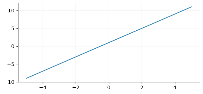
Fig. 48 The custom linear mean function evaluated on a linearly spaced grid of inputs, recovering the expected straight line.#
Looks good! To conclude this section, let’s now parameterise a GP with our new mean function and see how gradients may be computed.
y = jnp.sin(X)
D = gpx.Dataset(X, y)

prior = gpx.gps.Prior(mean_function=meanf, kernel=gpx.kernels.Matern32())
likelihood = gpx.likelihoods.Gaussian(D.n)
posterior = likelihood * prior
We’ll compute derivatives of the conjugate marginal log-likelihood
(conjugate_mll). With Equinox and
Paramax, this is straightforward: the loss takes the model exactly as it is, and
eqx.filter_value_and_grad computes gradients with respect to the array leaves —
which, as we saw above, are the parameters’ unconstrained internals. The bijections
are applied by the val calls inside the kernel, mean function and likelihood, so
they sit on the differentiated path and are accounted for by the chain rule
automatically.
def loss_fn(model, data: gpx.Dataset) -> ScalarFloat:
    return -gpx.objectives.conjugate_mll(model, data)


_, param_grads = eqx.filter_value_and_grad(loss_fn)(posterior, D)
In practice, you would wish to perform multiple iterations of gradient descent to
learn the optimal parameter values. However, for the purposes of illustration, we use
eqx.apply_updates in the below to update the model using its previously computed
gradients. As you can see, Equinox makes it easy to apply updates directly to the
model without manual split/merge operations.
LEARNING_RATE = 0.01
scaled_grads = jtu.tree_map(lambda g: LEARNING_RATE * g, param_grads)
optimised_posterior = eqx.apply_updates(posterior, scaled_grads)
Now we will plot the updated mean function alongside its initial form
(Fig. 49). Since the model
is updated in-place via eqx.apply_updates, we can simply invoke it as normal.
fig, ax = plt.subplots()
ax.plot(X, optimised_posterior.prior.mean_function(X), label="Updated mean function")
ax.plot(X, meanf(X), label="Initial mean function")
ax.legend()
ax.set(xlabel="x", ylabel="m(x)")
plt.show()
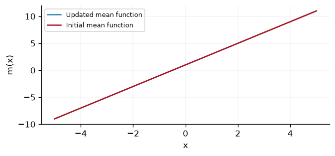
Fig. 49 The linear mean function before and after a single gradient step applied with eqx.apply_updates.#
Conclusions#
In this notebook we have explored how GPJax’s Equinox-based backend may be easily manipulated and extended. For a more applied look at this, see how we construct a kernel on polar coordinates in our Kernel Guide notebook.
System configuration#
%reload_ext watermark
%watermark -n -u -v -iv -w -a 'Thomas Pinder'
Author: Thomas Pinder

Last updated: Mon, 28 Sep 2026

Python implementation: CPython
Python version       : 3.11.16
IPython version      : 9.17.1

equinox   : 0.13.8
gpjax     : 1.0.0
jax       : 0.10.2
jaxtyping : 0.3.11
matplotlib: 3.11.2
myst_nb   : 1.4.0
paramax   : 0.0.5

Watermark: 2.6.0